Getting Started
deisa-dask is a lightweight integration layer that connects MPI-based HPC applications with the Dask distributed runtime.
It is part of the deisa ecosystem and is designed for in situ analysis workflows, where simulation codes directly offload computations to distributed Dask workers.
Unlike standalone Dask usage, deisa-dask is intended to run inside MPI-parallel applications on HPC systems, bridging tightly coupled simulation and distributed analytics.
Architecture Overview
deisa-dask acts as a bridge between:
- MPI simulation codes (C/C++/Fortran/Python, see PDI for more info)
- deisa core abstractions (data movement + orchestration layer)
- Dask distributed scheduler and workers
MPI ranks (simulation)
        │
        │  deisa interface
        ▼
deisa-dask layer
        │
        ▼
Dask scheduler + workers
        │
        ▼
Distributed analysis tasks
The key idea is that the simulation drives the execution, not the scheduler.
Prerequisites
deisa-dask is designed for HPC environments. You will typically need:
- Python ≥ 3.10
- MPI implementation (OpenMPI or MPICH)
- mpi4py
- dask
- distributed
- deisa-core
- Optional: SLURM (or another batch system)
Installation
deisa-dask can be installed in several ways depending on your environment.
Pip (Python environments)
pip install deisa-daskThis is the simplest option and suitable for local testing or Python virtual environments.
From source (development / bleeding edge)
git clone https://github.com/deisa-project/deisa-dask.git
cd deisa-dask
pip install -e .
Use this if you are:
- contributing to deisa-dask
- testing experimental MPI/Dask coupling features
- integrating with deisa development workflows
Spack (HPC package manager)
deisa-dask is available through Spack environments used in HPC deployments:
spack install py-deisa-dask
spack load py-deisa-dask
This is the recommended method on systems where:
- Python environments are centrally managed
- MPI and Python stacks are provided by Spack
- reproducibility across compute centers is required
Spack ensures consistent builds of:
mpi4pydaskdeisa-core- Python runtime dependencies
Guix / guix-science
deisa-dask is also available via the guix-science channel, enabling fully reproducible HPC environments:
guix install python-deisa-daskor inside a manifest:
(specifications->manifest
 '("python-deisa-dask"))
This approach is ideal for:
- reproducible research workflows
- long-term scientific reproducibility
- tightly controlled software stacks
Minimal Example: Local Dask Cluster
This example demonstrates the basic execution model of deisa-dask using MPI. It launches a local Dask scheduler and worker, starts an MPI simulation, and runs an analysis process that receives distributed arrays as Dask arrays.
The simulation generates a synthetic temperature field on four MPI ranks. At each timestep, every rank sends its local portion of the global array through the deisa bridge. The analysis application reconstructs the distributed array as a Dask array, computes its global sum, and saves a visualization of the latest timestep.
The complete example has the following structure:
.
└── example
   └── getting-started
       ├── analysis.py
       ├── launch.sh
       └── simulation.py
Steps
Simulation
The simulation is a simple MPI program running on 4 ranks arranged in a 2×2 Cartesian topology. Each rank owns one quarter of a 64×64 global grid.
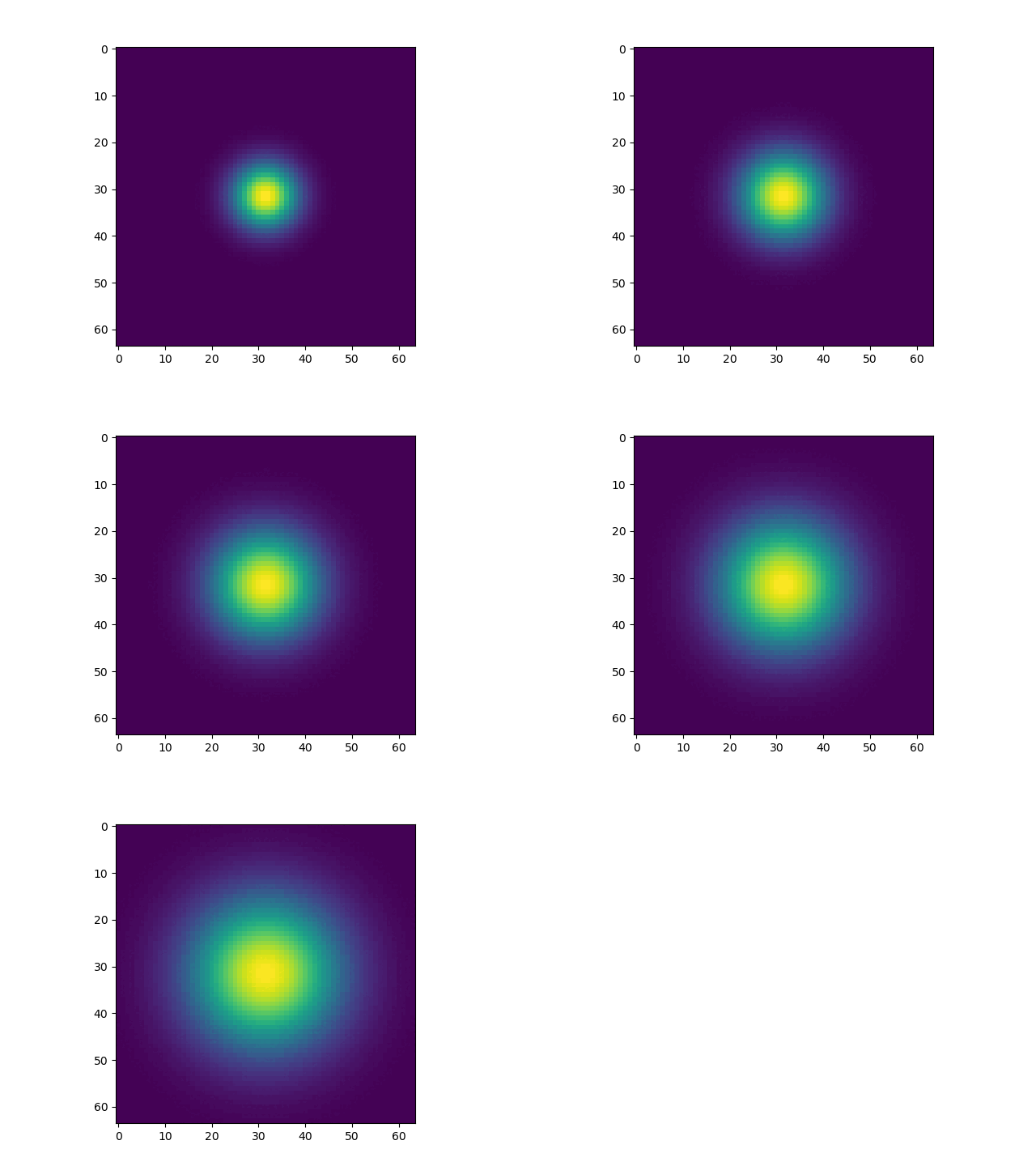
After creating the Bridge, the simulation repeatedly generates a synthetic Gaussian temperature field whose width increases over time.
Each MPI rank sends only its local subdomain using bridge.send().
The metadata provided when constructing the bridge describes how the local chunks are assembled into a global distributed array.
import numpy as np
from mpi4py import MPI

from deisa.dask import Bridge

global_grid_size = (64, 64)
mpi_parallelism = (2, 2)

comm = MPI.COMM_WORLD
rank = comm.Get_rank()
size = comm.Get_size()

assert size == 4, "This example requires 4 ranks"

print(f"[{rank}] Hello from simulation. comm size={size}")

dims = MPI.Compute_dims(size, len(global_grid_size))
cart_comm = comm.Create_cart(dims)
rank_coords = cart_comm.Get_coords(rank)

nx_local = global_grid_size[0] // mpi_parallelism[0]
ny_local = global_grid_size[1] // mpi_parallelism[1]

# indices for this rank
x_start = rank_coords[0] * nx_local
x_end = (rank_coords[0] + 1) * nx_local
y_start = rank_coords[1] * ny_local
y_end = (rank_coords[1] + 1) * ny_local

x_full = np.linspace(-1, 1, global_grid_size[0])
y_full = np.linspace(-1, 1, global_grid_size[1])

x_local = x_full[x_start:x_end]
y_local = y_full[y_start:y_end]

X, Y = np.meshgrid(x_local, y_local, indexing="ij")

# Start the Bridge
bridge = Bridge(
    comm=comm,
    arrays_metadata={
        "temperature": {
            "global_shape": global_grid_size,
            "chunk_shape": tuple(g // p for g, p in zip(global_grid_size, mpi_parallelism)),
            "chunk_position": rank_coords,
        }
    },
)

for ts in range(5):
    print(f"[{rank}] Sending timestep {ts}", flush=True)
    sigma = 0.15 + ts * 0.05
    local_data = np.exp(-(X**2 + Y**2) / (2 * sigma**2))
    bridge.send("temperature", local_data, timestep=ts)

bridge.close(timestep=5)
Analysis
The analysis process creates a Deisa instance and registers a callback for the temperature data.
Whenever new timesteps become available, deisa invokes the callback with a sequence of Dask arrays representing the received timesteps
(in this example, the temperature sliding window array is by default of size 1).
In this example, the callback:
- selects the most recent timestep,
- computes the global sum of the distributed array,
- renders the array using Matplotlib, and
- saves the image as
heat-<timestep>.png.
Because the data remain distributed as Dask arrays, operations such as sum() execute in parallel on the Dask worker.
from matplotlib.backends.backend_agg import FigureCanvasAgg
from matplotlib.figure import Figure

from deisa.dask import Deisa

deisa = Deisa()


@deisa.register("temperature")
def callback(temperatures):

    latest_temperature = temperatures[-1]
    # compute the sum of the latest temperature
    sum = latest_temperature.sum().compute()
    print(f"latest temperature t={latest_temperature.timestep}, sum={sum}", flush=True)

    # plot the latest temperature
    fig = Figure()
    FigureCanvasAgg(fig)
    ax = fig.add_subplot(111)
    ax.imshow(latest_temperature, cmap="viridis", interpolation="none")
    fig.savefig(f"heat-{latest_temperature.timestep}.png")
    fig.clear()


# wait for all tasks and for simulation to finish
deisa.execute_callbacks()
Launcher script
The launcher script starts all components required by the example in the correct order:
- a Dask scheduler,
- a Dask worker,
- the analysis process,
- the MPI simulation.
The simulation connects to the scheduler through the DEISA_DASK_SCHEDULER_ADDRESS environment variable.
Once the simulation finishes, the script waits for the analysis to process the remaining data before shutting down the worker and scheduler.
For simplicity, this launcher script runs everything on a single machine. In a production deployment, the scheduler, workers, simulation, and analysis may all execute on different nodes.
#!/usr/bin/env bash

export DEISA_DASK_SCHEDULER_ADDRESS="tcp://localhost:8786"

mpirun -np 1 dask scheduler --scheduler-file scheduler.json --protocol tcp --host localhost --port '8786' &
scheduler_pid=$!

sleep 5

mpirun -np 1 dask worker --scheduler-file scheduler.json &
worker_pid=$!

sleep 2

mpirun -np 1 python3 analysis.py &
analysis_pid=$!

mpirun -np 4 python3 simulation.py
simulation_pid=$!

echo "kill worker PID: $worker_pid"
kill $worker_pid
echo "waiting for worker, analysis and simulation PIDs to finish"
wait $worker_pid $analysis_pid $simulation_pid
echo "kill scheduler PID: $scheduler_pid"
kill $scheduler_pid

echo "launcher is done."
Results
Running the launcher script produces a sequence of images (heat-0.png to heat-4.png), one for each timestep received by the analysis application.
The animation below shows the reconstructed global temperature field. Although the simulation sends only local subdomains from each MPI rank, deisa automatically assembles them into a distributed Dask array. The analysis callback then computes on the global array and generates the visualization without requiring any explicit gather operation.
In this example, the Gaussian temperature field becomes progressively wider over time, demonstrating how timesteps are streamed from the simulation to the analysis process as they are produced.
The results are saved into the directory with the code like this:
.
└── example
   └── getting-started
       ├── analysis.py
       ├── launch.sh
       ├── simulation.py
       ├── heat-0.png
       ├── heat-1.png
       ├── heat-2.png
       ├── heat-3.png
       └── heat-4.png
From this, you can create this beautiful gif by executing
convert -delay 30 *.png heat.gifNOTE: This requires the use of
imagemagick, make sure you have it installed on your machine.
Next
Explore the following sections to start adding more contents: